Meaning is an orphan. A notion can be written, spoken, drawn, or conveyed by a sharp look that makes further scholarship quite unnecessary. These are entirely different phenomena. They arrive by means unalike and recent scholarship would have it that they are perceived very differently. And yet, something survives the journey enough for us to reconcile disparate messages into the same thing. And if said thing is something we need machines to understand, it seems very suspicious that the way to go about it is to divide the world into text, images and audio.
Modalities are a rather dubious concept in machine learning. It's quite possible that the way we understand them may be a principal reason we seem so close and yet so far from true intelligence. It has a certain promiscuity to it in that its meaning is highly mobile across at least 4 distinct readings.
The diagram distinguishes four meanings of modality. These are levels of description, rather than consecutive stages in a process.
- Physical substrate or transducer. What produced the signal? Examples include photons falling on a sensor and pressure waves reaching a microphone.
- Encoding. How is the data represented? Examples include a grid of floating point numbers, a sequence of discrete tokens, and a graph of nodes and edges.
- Statistical structure. What regularities does the data have? The diagram shows the same spatial pattern shifted one cell to the right, illustrating translation equivariance. It also shows the ordered tokens “the bird sings”, illustrating sequence order in text.
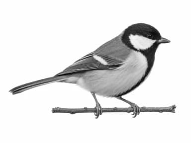
- Semantic domain. What is the data about? A generated picture of a songbird, a schematic bird call, and the sentence “a bird sings” share the same subject. The waveform is an illustration, not a recording of the pictured bird.
This seems hilariously vague the more you think about it. A spectrogram is audio on one level and an image on another. Text is image in one sense, audio in another, and something else entirely in your brain. Training frontier models seems to be a rather absurd endeavour in coaxing a machine to equivocate across these categories fluently.
This arose, perhaps, because we individuate the senses by organ, by stimulus, by phenomenological character or by content. Quine contends that our sorting of the world into kinds rests on an innate sense of similarity, a "quality space" that evolution tuned to our sensory apparatus that is good for induction. A great big accident of the primaeval ooze. Ordinary talk of the “senses” or “modalities” is about as well-defined as the rules of engagement in a sixteenth-century European skirmish.
You'll Know What We Did Last Summer(s)
20-25 year old Californian women
What does this actually represent? The trivial reading is that it is a sequence of symbols. The playbook here being training an embedding model to place these symbols in vector space close to where it similar statements co-occur. The more pretentious reading is that this is a distribution that can be represented by some Gaussian mixture.
The true and computationally intractable reading is that this represents a distribution where each sample is a person — with their own weights to support some hitherto undiscovered model of a singular person.
If you hold this reading (and we do), it doesn't make any sense to embed these symbols by statistically torturing existing text corpora. The immediate objection is that this is a very nice piece of navel-gazing, but a very poor experimental strategy to arrive at anything approximating a model.
Contrary to our own expectations, we did in fact arrive at a lot more than an embedding model a year later (see Giedi 2).
It Works in a Browser
Suppose we want to predict how a population would answer a survey. We might ask how the prediction changes if the population is older, if we consider only graduates, or if we combine two audiences in different proportions. Then we might ask an entirely different survey question. We would like to retain what the model already knows about the population through all of this, without requiring it to undertake a fresh demographic education every time someone changes the subject.
This is the application we have in mind. Encode a population, operate on its representation, then give the resulting vector to a model trained to answer the question we care about. Survey prediction, audience comparison and estimating demand for a service could all use this arrangement: the population supplies a common input, while each predictor learns its own task.
The small example below lets you try the population operations with the actual tiny model running in your browser. We supply two populations of 800 synthetic adults, with different age compositions. Blend them, keep the older adults, then keep the graduates. The model performs these operations on a sixteen-dimensional population vector; its statistical readout estimates how many people remain.
Population A 800 adults · 50% aged 50+
Population B 800 adults · 75% aged 50+
Run to update the counts.
Input Populations
| Demographic Cell | Population A | Population B |
|---|---|---|
| Women · 18–49 · no degree | 100 | 50 |
| Women · 18–49 · degree | 100 | 50 |
| Women · 50+ · no degree | 100 | 150 |
| Women · 50+ · degree | 100 | 150 |
| Men · 18–49 · no degree | 100 | 50 |
| Men · 18–49 · degree | 100 | 50 |
| Men · 50+ · no degree | 100 | 150 |
| Men · 50+ · degree | 100 | 150 |
| Total Adults | 800 | 800 |
Move the slider and press Run Experiment. Compare Model with Exact, then reverse the order of the restrictions: selecting older graduates should find the same people either way.
For these eight synthetic groups, we can calculate the answers exactly from the supplied counts, and ordinary arithmetic is entitled to question our expenditure. Its role here is to tell us how well the learned operations work. The coloured grids show the population state after each step; that state is also what we can hand to another model for a new prediction task. Whether we can teach those sixteen numbers to support both uses is the research question. The browser gives us a small working instance of the machinery; the experiments that follow examine how much it deserves our confidence.
The Art of the Possible
What would we expect the ideal embedding model for this task to do? Allow us to consensually pump your intuition so we can get you to our preferred conclusions.
Given some description of a demographic, , and our ideal encoder, , we have:
Statistics
As any human reader would, we would expect to have some statistical introspectability. After all, it is indeed an encoding of a very sophisticated distribution. Consider these:
- "20-25 year old Californian women" is a relatively large population. Even if you do not know the precise number, you would expect it to be greater than the number of 20 year old Californian women and lesser than the number of Californian women. This is elementary logic.
- A moderately informed person would further move abductively to conclude that there are probably less of them than there are Londoners, but not much less than there are Irishmen.
- A regrettable familiarity with California and a first-order encounter with the economy would further induce one to conclude that this population is very likely to be students, renters, unmarried, and presently not very happy with Vaswani et al.
These are things that are variously true by construction, reasonable expectations, and workable assumptions pending verification. This implies that should encode attributes in metric space required to support such inferences.
Algebra
A population is also a set that accomodates certain operations. We can reasonably conclude that would admit some Boolean algebra, counting, and some very sophisticated operations that are unique to collections of people.
- "20-30 year old Californian women" "20-25 year old Californian women" = "26-30 year old Californian women"
- A blend of 70% "20-25 year old Californian women" and 30% "26-30 year old Californian women" should support statistical inferences exampled in the previous set while reflecting the blend.
- Boolean logic should support the construction of sophisticated demographic subsets. "20-25 year old Californian women and 50-60 year old Eritrean women" is a high-variance subset — one half of which is of dubious construction owing to paucity of data.
Lastly, there is the semantic aspect of the matter that text embedding models already do quite well. California and Eritrea are very different places. In our ideal world, we retain that distinction whole.
Our question is precise enough to invite falsification now.
Can learned population vectors support statistical computation and help another model learn population-dependent tasks?
The principal artifact we would hope out of this research is an embedding model that is capable of taking descriptions of demographics and encoding them into a vector space that can support a hypothetical Large Population Model (LPM). That gives us two things to establish: whether the vectors support the computations we ask of them, and whether what they learn is of any use beyond those computations.
A Rather Small Encoder
The first point of comparison must of necessity be with existing embedding models.
Before asking our encoder to support more ambitious operations, we should establish whether its vectors are useful for learning about populations at all. We begin with a small text encoder as a base and compare it with MiniLM.
Some sense of proportion is helpful here. MiniLM is a 22M parameter model that uses deep self-attention. Our small encoder has 251K parameters, roughly one ninetieth as many, and produces a 96-dimensional embedding to MiniLM's 384. There was always reason to suspect that a smaller encoder would do. As the task is narrow in the more semantically rich space of text, it need only be proficient in encoding descriptions of populations. Gemma 2 2B spends almost 1/4th of its parameters on simply embedding information; but it has to contend with multilinguality, a much larger domain, and the need to support a wide range of tasks.
There are three training regimes from which we can source a model.
- Task-only training. The model trains only on the downstream task, without prior statistics or algebra training. This tests whether the additional training provides benefits beyond learning directly from task labels.
- Statistics training. The model is pretrained to support statistical computation, followed by training on the downstream task.
- Algebra training. The model is pretrained to support statistical computation, population operations, and responses to changed input facts, followed by training on the downstream task.
01
Task-only training
Task labels only
Downstream task training
02
Statistics training
Statistics pretraining
Downstream task training
03
Algebra training
Algebra pretraining
Downstream task training
We compare the statistics- and algebra-trained text encoders with MiniLM at predicting responses to survey questions from CES. For this comparison, the encoders are frozen and an affine readout is trained on each encoder's vectors. This tests their usefulness for population-dependent prediction.
Figure
Encoder size and survey-response error
Frozen encoders · 128 labelled groups
| Model | Encoder parameterslog₁₀ scale | MAE (pp)linear scale · lower is better |
|---|---|---|
| StatisticsPopulation Encoder / Text | 7.99 | |
| Statistics + AlgebraPopulation Encoder / Text | 8.03 | |
| MiniLM · 384 dimensions | 7.76 |
MiniLM uses 90.2× as many encoder parameters for 0.23 pp lower MAE than the statistics encoder.
Encoder parameters only · lower MAE is better
Study notes
96-dimensional text-only population encoders. Three source seeds and three label draws; dependent repeats do not add independent populations. MiniLM uses its full 384 dimensions. Differences in architecture and pretraining remain part of this reference comparison. Each model occupies one row. Encoder parameters use a shared logarithmic scale from 100K to 100M; validation percentage-point MAE uses a separate shared linear scale from zero to 10. Frozen encoders and affine readouts at 128 labelled groups. Population encoders have 251,712 parameters each; MiniLM has 22,713,216, including its pooler. The complete population source-training model has 408,175 parameters including auxiliary modules; the 90× ratio compares encoders. Points show observed models, not a fitted scaling relationship.
At 128 labelled groups, our statistics-trained encoder scores 7.99pp of mean absolute error against MiniLM's 7.76pp. The shortfall is a mere 0.23pp.
Delightfully, this proximity in performance carries over to changes in label budget. From 64 through 512 labelled groups, we never exceed 0.27pp of error. At 16 labels, both population pretraining conditions have slightly lower point estimates. MiniLM leads from 32 labels onward, but the shortfall remains vanishingly small.
Figure
Close across the label budgets
Frozen encoders · CES survey responses
MAE (percentage points)
Lower is better · vertical axis 7–10
| Model | MAE (pp)Labelled groups · lower is better | |||||
|---|---|---|---|---|---|---|
| 16 | 32 | 64 | 128 | 256 | 512 | |
| StatisticsPopulation Encoder / Text | 16 labelled contexts: 8.82 | 32 labelled contexts: 8.48 | 64 labelled contexts: 8.14 | 128 labelled contexts: 7.99 | 256 labelled contexts: 7.90 | 512 labelled contexts: 7.85 |
| Statistics + AlgebraPopulation Encoder / Text | 16 labelled contexts: 8.80 | 32 labelled contexts: 8.69 | 64 labelled contexts: 8.16 | 128 labelled contexts: 8.03 | 256 labelled contexts: 7.96 | 512 labelled contexts: 7.94 |
| MiniLM · 384 dimensions | 16 labelled contexts: 8.94 | 32 labelled contexts: 8.11 | 64 labelled contexts: 7.89 | 128 labelled contexts: 7.76 | 256 labelled contexts: 7.72 | 512 labelled contexts: 7.58 |
From 64 to 512 labels, the statistics encoder stays within 0.27 percentage points of MiniLM.
Study notes
96-dimensional text-only population encoders. Three source seeds and three label draws; dependent repeats do not add independent populations. MiniLM uses its full 384 dimensions. Differences in architecture and pretraining remain part of this reference comparison. Frozen affine probes use identical labelled groups and the same in-budget Ridge selection. Each point averages nine source-seed/label-draw fits. The horizontal axis doubles from 16 to 512 labels; the vertical axis spans 7–10 percentage points to resolve the small differences. Connecting lines guide the eye; they do not represent extra fits or uncertainty intervals. These are development validation results.
Finally, we can ask what hapens if we allow the small encoder to adapt to the downstream task. Doing so gives a similarly competitive picture. At 128 labels, statistics remains approx. 0.19pp behind a frozen MiniLM on held respondents with known combinations, and 0.28pp behind on held geography. On held combinations, statistics is about 0.18pp ahead. It's worth noting that algebra does not seem to furnish any consistent advantage on ordinary survey responses.
Figure
The small encoder remains competitive on held responses
128 labels · CES survey responses
Fine-tuned population encoders · frozen MiniLM
Blocks show differences between adjacent models.
| Model | Held respondentsknown combinationsMAE (pp) · lower is better | Held respondentsheld combinationsMAE (pp) · lower is better | Held geographyMAE (pp) · lower is better |
|---|---|---|---|
| StatisticsPopulation Encoder / Text | |||
| Statistics + AlgebraPopulation Encoder / Text | |||
| MiniLM · 384 dimensions |
| Model | Held respondentsknown combinationsMAE (pp) · lower is better |
|---|---|
| StatisticsPopulation Encoder / Text | |
| Statistics + AlgebraPopulation Encoder / Text | |
| MiniLM · 384 dimensions |
| Model | Held respondentsheld combinationsMAE (pp) · lower is better |
|---|---|
| StatisticsPopulation Encoder / Text | |
| Statistics + AlgebraPopulation Encoder / Text | |
| MiniLM · 384 dimensions |
| Model | Held geographyMAE (pp) · lower is better |
|---|---|
| StatisticsPopulation Encoder / Text | |
| Statistics + AlgebraPopulation Encoder / Text | |
| MiniLM · 384 dimensions |
At 128 labels, fine-tuned statistics is 0.19–0.28 pp behind MiniLM in two CES strata and 0.18 pp ahead on held combinations.
Point estimates · no equivalence claim
Study notes
96-dimensional text-only population encoders. Three source seeds and three label draws; dependent repeats do not add independent populations. MiniLM uses its full 384 dimensions. Differences in architecture and pretraining remain part of this reference comparison. Sealed CES response assessment, 128 labels and familiar wording; state-macro MAE averaged across nine fits. Population encoders are fine-tuned with the same reset MLP (267,232 adaptable parameters); MiniLM remains frozen with an affine readout. Respondent strata share assessment participants and uncertainty is clustered by state. These point estimates measure competitiveness on CES, not statistical equivalence or general cross-survey performance.
Developing the Population Representation
Of course, having now established that our more specialized encoder fares decently against a much larger model at more superficial tasks, we must set ourselves to the question of precisely what it is that these "improvements" are doing for us.
What does statistics pretraining add? Does explicitly teaching operations add anything?
To answer this question, we invent populations with exactly-known compositions. Each composition has eight groups formed by combining sex, age band, and degree status. A singular example would, to give an illustrative one, say, "blend these two populations, then keep adults aged 50 or older." We further provide numerical facts about the original populations and an operation. It must then represent the resulting population well enough for a small predictor to estimate four quantities:
- Mean event risk: invented group-specific event probabilities.
- Risk variance: how much those probabilities differ between people.
- Profile entropy: how evenly the population is spread across its eight groups.
- Expected event count: a population-size-dependent total under a second invented event law.
Note that these are entirely contrived mathematical targets, with no measurable in the real world. We freeze our encoder, train a small 676-parameter prediction head using 128 labelled population contexts, then evaluate on 512 held-out ones. The graphic below averages across 3 seeds and three label draws.
Figure
What pretraining contributes
Frozen encoders · 128 labelled contexts
Shared linear scale: 0.07–0.10 · axis starts above zero. Blocks show differences between training regimes.
| Training regime | Population Encoder / Contextual16-dimensional vectorsFact-sensitive MAELower is better | Population Encoder / Independent16-dimensional vectorsFact-sensitive MAELower is better |
|---|---|---|
| Task only | ||
| Statistics only | ||
| Statistics + algebra |
| Training regime | Population Encoder / Contextual16-dimensional vectorsFact-sensitive MAELower is better |
|---|---|
| Task only | |
| Statistics only | |
| Statistics + algebra |
| Training regime | Population Encoder / Independent16-dimensional vectorsFact-sensitive MAELower is better |
|---|---|
| Task only | |
| Statistics only | |
| Statistics + algebra |
Statistics and algebra teaching each improve the earlier frozen-consumer comparison.
Synthetic tasks · point estimates · input access and capacity differ across architectures
Study notes
Earlier contextual18 and independent9 models: 16-dimensional vectors from text plus supplied population facts. Frozen encoders; new 676-parameter heads at 128 labelled contexts. Task only uses a random frozen encoder. Composite error covers synthetic risk, risk variance, entropy and event count, not CES responses. Three source seeds; input access and capacity differ across architectures.
Statistics training reduces error by 10.17% for Contextual and 8.66% for Independent, relative to their random-feature controls. Algebra adds a further 6.57% and 13.68% reduction, respectively.
Does teaching individual operations produce reliable sequences?
Of course, it should strike you that an embedding that is capable of supporting a single algebraic operation may be too shallow to support multiple algebraic operations. This is, we could even speculate, a limitation that will plague us on account of the nature of floating point independent of how many clever tricks we employ in the construction of the embedding.
It's difficult to test general sequence reasoning for a number of reasons we won't go into here. We can attempt smaller, more developmental diagnostics that give us an idea of the direction but not necessarily the scope of improvement. We again take populations of 8 groups. Each group contains 200, 400, 800 or 1200 people, distributed randomly among those groups. The model receives a population description, eight group proportions and their scaled counts. Our encoder processes it to a 16-dim vector. A learned operator then changes those numbers when instructed to restrict or blend populations. Finally, the previously designed statistical readout predicts population size.
Figure
From individual operations to sequences
Earlier population encoders · development
| Operation | Count MAE (people)Linear scale · lower is better | StatisticsPopulation Encoder / Independent | Statistics + AlgebraPopulation Encoder / Independent |
|---|---|---|---|
| One restriction | 324.62 | 97.32 | |
| Two restrictions | 476.41 | 89.70 | |
| Five restrictions | 979.00 | 96.35 | |
| One blend | 527.61 | 101.71 | |
| Repeated blends | 487.00 | 110.67 | |
Algebra teaching reduces sequence errors, while success on repeated steps remains a limited test.
Three seeds · 64 reused validation contexts · source-trained readouts
Study notes
Earlier independent9 source encoders; three seeds on 64 reused validation contexts. These are source-trained readouts, not a fresh sequence-generalization claim.
The resulting score is a mean absolute population-count error, measured in people. Operation training substantially reduces error in every class. It also keeps the 5-restriction error close to single-restriction error. However, as can be seen quite readily in the figure, the error is still quite significant. The finding here remains that training our encoder in explicit operations makes these learned operators a lot more usable for repeatedly stacking operations.
Man proposes, gradient descent — that unfeeling golden god — disposes. An apparent capacity to meet our requirement to produce the capabilities we demand of it may simply be a lookup table of exceptional size and trickery.
Here we hold the population facts and operations fixed, then express the same task in two different ways. One uses the construction that is known through training and the other changes the wording.
The wording comparison sneaks in the final H-Algebra model (the construction of which will be discussed soon). Its training includes correct answers under two sets of supplied facts and the difference between those answers. We will discuss what this extra supervision actually buys us.
Figure
Accuracy under two supplied wordings
H-Algebra · fresh native evaluation
Count MAE (people) · lower is better · point estimates
- Algebra + ChangePopulation Encoder / H
| Query type | Count MAE (people)Linear · lower is better · point estimates | Wording 1 | Wording 2 |
|---|---|---|---|
| Direct query | 32.46 | 46.00 | |
| Held description | 51.44 | 57.38 | |
| One restriction | 29.85 | 31.23 | |
| Alternating operations | 15.35 | 19.76 |
Both wording variants are scored separately; similar averages alone do not prove paraphrase invariance.
Study notes
Three source seeds (17, 7, 29); 512 synthetic context pairs per cohort. Wordings and programs are dependent views, not additional independent populations. Ordinary cohort; homogeneous algebra model. This chart measures answer accuracy, not paired agreement between wordings. Some reserved constructions had earlier development exposure.
The two wordings have broadly similar errors for restrictions and alternating operations, with larger differences on direct queries. These are errors against the correct answer for each wording; they do not measure whether the two predictions agree. Nor are all the reserved constructions entirely untouched by earlier development. This is a useful wording diagnostic, with rather less entitlement to the word "invariance" than we might have liked.
Does a population's representation depend on irrelevant reference populations?
If our model was feeling particularly parsimonious, it could theoretically build an internal representation that is ill-formed. It would be task-effective but model its world in such a way that it is incapable of separating populations. In this case, the defect would manifest in a failure to answer questions about population A if facts about population B were to be perverted in some way.
Return now to the earlier encoders. If we ask about population A, changing facts about an unrelated population B should leave the answer alone. Our Contextual encoder receives the description and both reference tables. Our Independent encoder receives the description and only the selected reference's facts. These are the two architectures in the earlier pretraining comparison.
The distinction matters. Under statistics training, changing B moves Contextual's predicted count for A by about 81 people on average. Adding algebra training raises that to about 95.
Figure
Changing the other population
Earlier population encoders · development
Unwanted change in population A (people)Absolute predicted count change · linear · lower is better
| Training condition | Unwanted change in population A (people)Absolute count change · linear · lower is better | Population Encoder / Contextual | Population Encoder / Independent |
|---|---|---|---|
| Statistics only | Population Encoder / Contextual81.39 | Population Encoder / Independent0.00 | |
| Statistics + algebra | Population Encoder / Contextual94.97 | Population Encoder / Independent0.00 |
The independent interface removes partner-reference sensitivity by construction.
Zero sensitivity does not establish correct demographic selection.
Three seeds · reused development contexts · point estimates
Study notes
Earlier source encoders; mean over three seeds on reused development contexts. Zero sensitivity is imposed by the independent input interface; it does not establish correct demographic selection.
Independent has zero partner sensitivity because B's facts never enter its computation. This is a rather satisfying problem to solve by declining to give the model an opportunity to have it. It doesn't tell us whether the answer about A is correct. For that, we must ask whether the model uses the information that does belong to A.
Is our model committing a fallacy of division? Two populations could have identical demographic percentages but different combinations of characteristics. The model should ideally be able to distinguish these differences.
The concern here is a related error of inferring intersections from aggregate facts. In a population of 100 people, knowing that 50 are women and 50 are graduates tells us remarkably little about how many are women with degrees. It could be none; it could be all 50. A representation that retains each percentage while losing their association has discarded something necessary for selection.
Our diagnostic is stricter than this example. We change the eight-cell joint distribution while holding the total and all one- and two-way margins fixed. Only the three-way association changes. The model receives the changed facts; we ask whether a new predictor built on its frozen vectors changes its answer by the correct amount. A predictor that ignores the intervention gives us a useful no-change reference.
Figure
Changing joint facts while preserving margins
Earlier encoders · post-hoc joint diagnostic
Changed-answer error
Joint-controlled change MAE · lower is better · linear scale
| Model / condition | Observed error | Value |
|---|---|---|
| Task only | ||
| Predicted change | 0.02187 | |
| No-change reference | 0.0219 | |
| Statistics only | ||
| Predicted change | 0.02203 | |
| No-change reference | 0.0219 | |
| Statistics + algebra | ||
| Predicted change | 0.02229 | |
| No-change reference | 0.0219 | |
Supplying joint facts does not ensure that a new readout responds correctly.
Post-hoc diagnostic · earlier independent encoder · not H-Algebra results
Study notes
Earlier independent9 frozen consumers on mixed programs, 128 labels. One- and two-way margins and totals stay fixed. These post-hoc diagnostics reuse the earlier final cohort and are not H-Algebra results.
At 128 labels, all three training regimes are close to that reference, and statistics and algebra have slightly worse point estimates. Ordinary prediction improvements have not bought us a convincing response to joint information. These are post-hoc diagnostics on the earlier cohort, but they identify a concrete weakness worth addressing.
Does explicitly teaching factual changes improve that response?
Showing a model two correct facts may not teach the model how a change in the facts connects them. If we teach that explicitly, will that improve performance?
We add a loss on the difference between the answers under paired factual views, alongside teaching each answer separately. The architecture stays fixed. The training now asks the model to account for movement between two populations, as well as for their endpoints.
Figure
Teaching the difference between factual views
Joint-fact teaching · source pilot
Joint-profile change error
Profile-change MAE · lower is better · linear scale
| Model / condition | Observed error | Value |
|---|---|---|
| One restriction | ||
| Endpoint teaching | 0.06114 | |
| + Change teaching | 0.05391 | |
| No-change reference | 0.06705 | |
| Two restrictions | ||
| Endpoint teaching | 0.09244 | |
| + Change teaching | 0.08633 | |
| No-change reference | 0.06544 | |
| Five restrictions | ||
| Endpoint teaching | 0.08309 | |
| + Change teaching | 0.07119 | |
| No-change reference | 0.06435 | |
| One blend | ||
| Endpoint teaching | 0.008801 | |
| + Change teaching | 0.008195 | |
| No-change reference | 0.0625 | |
| Repeated blends | ||
| Endpoint teaching | 0.008464 | |
| + Change teaching | 0.007565 | |
| No-change reference | 0.0625 | |
Explicit change teaching helps some operation families; the no-change reference remains essential.
One source seed · reused validation contexts · pilot comparison
Study notes
One seed (17), 64 reused validation contexts; matched sampling and encoder-forward budgets. No independent confirmation or new-head result is claimed by this pilot.
The one-seed pilot lowers profile-change error in every displayed operation family. Yet two and five restrictions still do worse than predicting no change. Improvement over a previous model and evidence that the new model follows the facts are distinct accomplishments. This pilot gives us reason to retain change supervision, with little reason to declare the matter settled.
Do separately predicted statistics agree with one another?
In the wild, the model will invariably see contradictory information. This is a feature of reality it must contend with. But is the model itself internally consistent? It is conceivable to have a model that is quite accurate in 80% of evaluation items while the remaining 20% represents a rather dramatic failure to reconcile its own internal representations. These would be trivial errors and inconsistencies in cell counts, total counts, and proportions.
Our synthetic populations spare us contradictory evidence. Any disagreement between their predicted totals, cell counts and proportions is therefore entirely the model's own contribution.
Figure
When separate statistical answers disagree
Earlier population encoders · development
Count versus decoded cell total
Mean absolute disagreement (people) · lower is better · linear scale
| Model / condition | Observed error | Value |
|---|---|---|
| Statistics only | ||
| Population Encoder / Contextual | 369 | |
| Population Encoder / Independent | 358.98 | |
| Statistics + algebra | ||
| Population Encoder / Contextual | 45.68 | |
| Population Encoder / Independent | 45.85 | |
Profile normalization
Mean absolute deviation from sum = 1 · lower is better · linear scale
| Model / condition | Observed error | Value |
|---|---|---|
| Statistics only | ||
| Population Encoder / Contextual | 0.8102 | |
| Population Encoder / Independent | 0.7943 | |
| Statistics + algebra | ||
| Population Encoder / Contextual | 0.06033 | |
| Population Encoder / Independent | 0.06175 | |
Algebra teaching reduces disagreement, but independently decoded statistics still need not reconcile.
Internal inconsistency · not accuracy against the population oracle
Study notes
Earlier encoders; three source seeds and reused development cases across direct queries and five operation families. Both panels measure internal inconsistency rather than accuracy against the population oracle.
Algebra training substantially reduces the disagreement. But the predicted total still differs from the sum of predicted cell counts by about 46 people on average in both earlier architectures. Separate readouts are being asked to discover a relationship we already know exactly.
Consider the model predicting a population of 100 people, and then giving us subgroup counts that add up to 120. Somewhere, somehow, twenty people were spontaneously ushered into existence. We could prevent this by having the model predict the subgroup counts first, and then arrive at a total.
This leads us to a mass representation. A single bias-free linear decoder maps the population vector to eight cell masses. We obtain the total by summing them and, for a positive total, obtain proportions by division. The statistics now share an arithmetic origin. They can still be wrong, but they cannot independently invent incompatible totals.
Can population operations work on a learned mass representation?
We can also design the model so that blending embeddings blends their predicted counts in the same proportions. For a linear count decoder and blend weight ,
Blending becomes a fixed weighted sum of vectors. Restriction remains learned: an instruction selects a linear transformation of the population state. It must learn which mass to retain, but its action on that state is constrained.
Figure
Restrictions on a learned mass state
Measure operators · source pilot
Count errors after operations
Count MAE (people) · lower is better · linear scale
| Model / condition | Observed error | Value |
|---|---|---|
| One restriction | ||
| Nonlinear restriction | 97.59 | |
| Linear restriction | 94.63 | |
| Two restrictions | ||
| Nonlinear restriction | 82.9 | |
| Linear restriction | 69.05 | |
| Five restrictions | ||
| Nonlinear restriction | 135.39 | |
| Linear restriction | 104.52 | |
| One blend | ||
| Nonlinear restriction | 10.94 | |
| Linear restriction | 6.84 | |
| Repeated blends | ||
| Nonlinear restriction | 10.95 | |
| Linear restriction | 7.64 | |
Linear restrictions improve several count errors in this matched pilot.
One source seed · reused validation contexts · pilot comparison
Study notes
One seed (17); pointwise teaching, 1,000 updates and 64 reused validation contexts. Both conditions use measure-state decoding. This is a comparison within the pilot, not against earlier probability-state models.
In a matched one-seed pilot, linear restrictions reduce two-restriction count error from about 83 to 69 people, and five-restriction error from 135 to 105. Both variants already use the mass decoder and fixed blending. This comparison supports the choice of restriction operator within that design; it does not isolate the benefit of the whole mass architecture against every earlier encoder.
Does explicitly teaching algebraic laws improve execution?
Rather surprisingly, idempotency is difficult for models to learn. In many cases, it has to be jackhammered into the training data so it can be learnt in the first place. Selecting older adults twice should not be any different from selecting them once. Selecting graduates, then older adults should be no different from selecting them in the opposite order.
We test an additional penalty for these laws and for complementary partitions: the masses selected by a condition and its complement should add back to the original. It is an appealing prescription. The model would presumably benefit from being told how to behave.
Figure
Does extra law supervision help?
Explicit algebra laws · fresh confirmation
- Algebra + ChangePopulation Encoder / Original
- Algebra + Change + LawsPopulation Encoder / Original
● Meets support rule○ Does not meet rule
Bonferroni-adjusted paired-world bootstrap intervals, conditional on fitted models. Support also requires improvement in every source seed.
Adding the law penalty
Error reduction (%) · right is better · linear axis -15% to 30%
| Comparison | Adjusted interval | Reduction |
|---|---|---|
| Mixed operations vs algebra without law loss | -5.38% | |
| Three distinct restrictions vs algebra without law loss | +2.04% | |
| Joint-fact response vs algebra without law loss | -9.53% | |
| Empty groups vs algebra without law loss | +24.02% |
Exact intervals and source-seed effects
- Mixed operations vs algebra without law loss
- Reduction: -5.377907972142109%. Adjusted interval: -6.589299556462495% to -4.134474267170726%. Source-seed effects: 6.637459562455033%, -5.749248955329101%, -18.598478870625428%. Does not meet support rule.
- Three distinct restrictions vs algebra without law loss
- Reduction: 2.0418485601621823%. Adjusted interval: -2.51176819682869% to 6.417115389466%. Source-seed effects: 19.19989509920619%, 8.064714395490228%, -26.407236946179%. Does not meet support rule.
- Joint-fact response vs algebra without law loss
- Reduction: -9.530329641805446%. Adjusted interval: -10.588753330997239% to -8.470128656978483%. Source-seed effects: -1.331548056164761%, -16.511845289964626%, -11.608943308903164%. Does not meet support rule.
- Empty groups vs algebra without law loss
- Reduction: 24.021343586385623%. Adjusted interval: 21.52917778267674% to 26.47827952341854%. Source-seed effects: 54.0791281533137%, 15.290683673612119%, -0.08710852530135411%. Does not meet support rule.
None of the four law-loss versus algebra comparisons meets the registered support rule.
Study notes
Three source seeds on fresh synthetic populations; candidate adds explicit law penalties. Whiskers are Bonferroni-adjusted paired-world bootstrap intervals, conditional on the fitted models. Support also requires improvement in every source seed. Filled points meet both criteria; hollow points do not.
None of the four comparisons meets the study's support rule. Mixed-operation and joint-response errors worsen on average. Empty-group error improves by about 24%, but one of the three source seeds reverses direction. The explicit law penalty does not earn its place in the final model.
Here and in the later interval plots, support requires both a positive multiple-comparison-adjusted interval and improvement in every source seed. The intervals resample paired synthetic worlds conditional on the fitted models; they do not measure all the uncertainty in retraining a model. An attractive average alone is insufficient.
From Size Scaling to H-Algebra
While text embedding models are content to place their embeddings on a unit sphere, magnitude is a valuable axis of information for us to retain in some capacity. A village and a city may have identical proportions, but their counts should differ by several orders of magnitude.
Does the mass representation behave correctly outside its training sizes?
Giving a model population size as an input does not ensure that it learns the required scaling. When we move to much smaller or larger populations, we may discover that it has learnt a tolerable approximation within its training range and very little arithmetic beyond it.
This brings about a rather trivial intervention. If we expect our vector to represent population mass, doubling a population while preserving composition should actually double the vector.
We ask the original mass model to encode each population at a fixed reference size of 1,200, preserving its composition, then multiply the resulting vector by the actual root size divided by 1,200. We call this inference-scaled algebra. No weights change. Since decoding and the instruction-conditioned restriction operators are linear in the population state, this route makes their outputs scale with root size as well.
Figure
A size repair using unchanged weights
Inference scaling · native confirmation
● Meets support rule○ Does not meet rule
Bonferroni-adjusted paired-world bootstrap intervals, conditional on fitted models. Support also requires improvement in every source seed.
Inference scaling versus original encoding
Error reduction (%) · right is better · linear axis -10% to 100%
| Comparison | Adjusted interval | Reduction |
|---|---|---|
| Small-size mixed operations vs original algebra | +96.63% | |
| Large-size mixed operations vs original algebra | +52.75% | |
| Ordinary mixed operations vs original algebra | +0.651% |
Exact intervals and source-seed effects
- Small-size mixed operations vs original algebra
- Reduction: 96.63206675149107%. Adjusted interval: 96.18926829750376% to 97.04347130470842%. Source-seed effects: 96.54160146556563%, 96.85023620698188%, 96.50134533235745%. Meets support rule.
- Large-size mixed operations vs original algebra
- Reduction: 52.75350312059518%. Adjusted interval: 51.45783103670307% to 53.891960292087695%. Source-seed effects: 46.52370602900493%, 56.35180338431813%, 54.96471004801475%. Meets support rule.
- Ordinary mixed operations vs original algebra
- Reduction: 0.6509947123511576%. Adjusted interval: -2.9476819020304195% to 4.2793177250495935%. Source-seed effects: 1.9136405019181044%, 2.3648346555822504%, -2.518745429951677%. Does not meet support rule.
Inference scaling greatly reduces small- and large-size count errors.
Study notes
Original algebra weights before and after reference-mass routing; separate earlier confirmation cohort. Whiskers are Bonferroni-adjusted paired-world bootstrap intervals, conditional on the fitted models. Support also requires improvement in every source seed. Filled points meet both criteria; hollow points do not.
The intervention reduces small-size count error by 96.63% and large-size error by 52.75% in the earlier confirmation cohort. Ordinary-size improvement is unsupported. A remarkably large portion of the extrapolation problem was amenable to multiplication.
Does that inference repair generalise, and what does it sacrifice?
This repair may be our undoing though. Scaling the vector could perturb relationships that the model needs to interpret demographic facts.
Figure
What the inference repair sacrifices
Inference scaling · native confirmation
● Meets support rule○ Does not meet rule
Bonferroni-adjusted paired-world bootstrap intervals, conditional on fitted models. Support also requires improvement in every source seed.
Benefits and regressions
Error reduction (%) · right is better · linear axis -25% to 40%
| Comparison | Adjusted interval | Reduction |
|---|---|---|
| Held-description count vs original algebra | +29.05% | |
| Three distinct restrictions vs original algebra | +29.4% | |
| Joint-fact response vs original algebra | -16.43% | |
| Empty groups vs original algebra | +33.09% |
Exact intervals and source-seed effects
- Held-description count vs original algebra
- Reduction: 29.0478583925763%. Adjusted interval: 23.693167651195466% to 34.47446821914654%. Source-seed effects: 43.89630879720411%, 13.29914822815447%, 14.140110178068351%. Meets support rule.
- Three distinct restrictions vs original algebra
- Reduction: 29.39824491446128%. Adjusted interval: 24.20821281194449% to 34.82915698752928%. Source-seed effects: 28.883240321478702%, 32.261099316240376%, 26.671534873082898%. Meets support rule.
- Joint-fact response vs original algebra
- Reduction: -16.434011083646453%. Adjusted interval: -21.92334648684424% to -11.361777612802406%. Source-seed effects: -19.673882186474188%, -10.261683510263135%, -18.81963609415767%. Does not meet support rule.
- Empty groups vs original algebra
- Reduction: 33.089737287866086%. Adjusted interval: 29.402588761405074% to 36.896903278814165%. Source-seed effects: 34.10801618347277%, 31.18557818667605%, 33.66794743001409%. Meets support rule.
Size repair comes with worse joint-fact response on the same frozen weights.
Study notes
Earlier inference-scaling confirmation. Joint response measures profile-change error; the other endpoints measure counts. All are shown as relative error reductions. Whiskers are Bonferroni-adjusted paired-world bootstrap intervals, conditional on the fitted models. Support also requires improvement in every source seed. Filled points meet both criteria; hollow points do not.
Held-description counts, three distinct restrictions and empty groups improve, but joint-fact response error grows by 16.43%. We have repaired size behaviour while making the model worse at responding to a change in composition. This is an awkward bargain for a population representation.
The model is, unfortunately, trained under one arrangement and then unceremoniously obliged to operate under a different one. In homogeneous training, reference-size encoding and explicit scaling are first-class citizens from initialization. This, combined with statistics, operation and factual-change training, constitutes H-Algebra. The explicit algebraic-law penalty is omitted.
For description , eight joint proportions , root size and reference size , its encoding has the form
The learned function constructs a representation at reference size; the explicit multiplier supplies its mass. During training, the model must now learn composition and operations in the same arrangement it will use at inference.
Figure
Homogeneous training reduces prediction error
H-Algebra · fresh native evaluation
Mixed operations at familiar population sizes
Cell-count MAE (people per cell) · lower is better · linear scale
| Model / condition | Observed error | Value |
|---|---|---|
| Algebra + ChangePopulation Encoder / Original | 16.29 | |
| Algebra + ChangePopulation Encoder / Scaled | 16.43 | |
| Algebra + ChangePopulation Encoder / H | 5.59 |
H-Algebra lowers cell-count error from 16.43 to 5.59 people per cell versus inference scaling: a 65.97% reduction.
Three source seeds · dependent views do not add independent populations
Study notes
Three source seeds (17, 7, 29); 512 synthetic context pairs per cohort. Wordings and programs are dependent views, not additional independent populations. All three models evaluate mixed operations on fresh populations at familiar sizes, rather than the small- and large-size extrapolation cohorts. Points show mean absolute error in predicted cell counts. Original and inference-scaled conditions reuse source weights; H-Algebra was trained with homogeneous routing from initialization.
At familiar sizes, mixed-operation cell-count error falls from 16.43 people per cell under inference scaling to 5.59 with H-Algebra, a 65.97% reduction. This is a comparison of training routes at ordinary sizes. We still need to establish what survives changes in size, composition, wording and operation sequence.
H-Algebra Tiny Architecture
H-Algebra Tiny is the architecture behind Giedi Embedding 0.1-tiny. In the experiments and plot labels, H-Algebra names its fully trained configuration. The resulting mass model has 252,787 parameters and a 16-dimensional state. A small two-layer Transformer encodes the text. A fusion network combines its output with the selected reference population's eight joint proportions and a fixed reference-size input. The explicit size multiplier then produces the population vector.
H-Algebra Tiny
Algebra + ChangePopulation Encoder / HTrained from tokens · 16-dimensional state
Both Transformer blocks have the expanded structure shown above, with independent weights. Each normalizes its input before attention and before the feed-forward network; the bypass paths add each sublayer’s input back to its output. is the token count. Dropout uses during training. Neuron marks in the fusion network are schematic; the labeled layer widths are exact. The final size scaling doubles the vector when the population doubles at fixed composition.
Restrictions apply instruction-conditioned linear operators to that state; blends take weighted sums. The shared linear mass decoder supplies cell counts, from which totals and proportions follow. The state can also be handed to a new model without the native statistical readout.
There is a considerable qualification to the phrase "embedding model" here. Unlike the text-only encoder compared with MiniLM, H-Algebra receives numerical facts about its reference population. It learns to represent and operate on supplied facts. It does not conjure a demographic census from a sentence. In our eight-cell world, exact table arithmetic is available throughout; it supplies the answers against which we judge the learned representation.
What Survived the Examination
What can the resulting H-Algebra model reliably execute?
Once we have a candidate model, we should look beyond its most flattering anecdotes. We should:
- ask direct statistical questions;
- execute mixed sequences;
- change the supplied facts;
- vary population sizes;
- introduce sparse populations;
- and use unfamiliar mixture weights.
The final native evaluation uses three trained seeds and 512 synthetic context pairs per cohort. Alternative wordings and programs are views of those same populations, so they do not multiply the number of independent examples. Here native means execution using the source model's own operators and statistical decoder. A new predictor consuming the vector is a separate examination.
Figure
Mixed operations and held descriptions
H-Algebra · fresh native evaluation
Mixed operations
Cell-count MAE (people per cell) · lower is better · linear scale
Ordinary mixed operations
| Model / condition | Observed error | Value |
|---|---|---|
| Algebra + ChangePopulation Encoder / H | 5.59 | |
| Algebra + ChangePopulation Encoder / Scaled | 16.43 |
Held descriptions
Total-count MAE (people) · lower is better · linear scale
Held-description count
| Model / condition | Observed error | Value |
|---|---|---|
| Algebra + ChangePopulation Encoder / H | 51.44 | |
| Algebra + ChangePopulation Encoder / Scaled | 61.92 |
H-Algebra improves cell-count error by 65.97% and held-description total-count error by 16.92% versus inference scaling.
Three source seeds · dependent views do not add independent populations
Study notes
Three source seeds (17, 7, 29); 512 synthetic context pairs per cohort. Wordings and programs are dependent views, not additional independent populations. Different units are kept in separate panels. These are the registered endpoint means, averaged over seeds.
Alongside the mixed-operation improvement, held-description total-count error falls from 61.92 to 51.44 people relative to inference scaling. These are different quantities: the first averages errors across eight cells, while the second measures the error in a population total. Their numerical scales should not be mistaken for a ranking of difficulty.
Figure
Joint facts across population sizes
H-Algebra · fresh native evaluation
- Algebra + ChangePopulation Encoder / H
- Algebra + ChangePopulation Encoder / Scaled
● Meets support rule○ Does not meet rule
Bonferroni-adjusted paired-world bootstrap intervals, conditional on fitted models. Support also requires improvement in every source seed.
H-Algebra versus inference scaling
Error reduction (%) · right is better · linear axis 0% to 80%
| Comparison | Adjusted interval | Reduction |
|---|---|---|
| Joint facts · familiar sizes vs inference scaling | +72.75% | |
| Joint facts · new sizes vs inference scaling | +73.22% |
Exact intervals and source-seed effects
- Joint facts · familiar sizes vs inference scaling
- Reduction: 72.75410836168534%. Adjusted interval: 71.51479656901697% to 73.92511265159128%. Source-seed effects: 77.48639678211732%, 58.19827149273037%, 80.39034197144638%. Meets support rule.
- Joint facts · new sizes vs inference scaling
- Reduction: 73.2187614658355%. Adjusted interval: 71.91227253675734% to 74.39935834203271%. Source-seed effects: 78.6751609003575%, 57.52861232194664%, 80.96036099043266%. Meets support rule.
Joint-fact response improves by about 73% versus inference scaling at familiar and new sizes.
Study notes
Three source seeds (17, 7, 29); 512 synthetic context pairs per cohort. Wordings and programs are dependent views, not additional independent populations. Interventions change a three-way association while holding size and lower-order margins fixed. Whiskers are Bonferroni-adjusted paired-world bootstrap intervals, conditional on the fitted models. Support also requires improvement in every source seed. Filled points meet both criteria; hollow points do not.
The joint-fact test is particularly encouraging. Relative to inference scaling, H-Algebra reduces profile-change error by about 73% at both familiar and unfamiliar sizes. Training in the homogeneous arrangement avoids the factual-response regression of the inference-only intervention.
Figure
Small and large populations
H-Algebra · fresh native evaluation
Small populations
Cell-count MAE (people per cell) · lower is better · linear scale
| Model / condition | Observed error | Value |
|---|---|---|
| Algebra + ChangePopulation Encoder / H | 0.3505 | |
| Algebra + ChangePopulation Encoder / Original | 24.97 | |
| Algebra + ChangePopulation Encoder / Scaled | 1.11 |
Large populations
Cell-count MAE (people per cell) · lower is better · linear scale
| Model / condition | Observed error | Value |
|---|---|---|
| Algebra + ChangePopulation Encoder / H | 62.9 | |
| Algebra + ChangePopulation Encoder / Original | 416.19 | |
| Algebra + ChangePopulation Encoder / Scaled | 186.11 |
Large relative improvements still leave visible absolute error at large sizes.
Three source seeds · dependent views do not add independent populations
Study notes
Three source seeds (17, 7, 29); 512 synthetic context pairs per cohort. Wordings and programs are dependent views, not additional independent populations. Small root sizes: 3, 11, 37, 113. Large root sizes: 3,200, 6,400, 12,800. Each panel has its own linear axis.
At root sizes of 3, 11, 37 and 113, mean cell-count error is about 0.35 people. At sizes of 3,200, 6,400 and 12,800 it is about 62.90. The relative gains over original algebra are large, but a model that scales its predictions also scales its mistakes. Homogeneity secures the size relationship; it does not make an imperfect composition estimate exact.
Figure
Sparse populations and new blend weights
H-Algebra · fresh native evaluation
Mixed-operation cell errors
Cell-count MAE (people per cell) · lower is better · linear scale
| Model / condition | Observed error | Value |
|---|---|---|
| Sparse populations | ||
| Algebra + ChangePopulation Encoder / H | 9.13 | |
| Algebra + ChangePopulation Encoder / Original | 30.57 | |
| Algebra + ChangePopulation Encoder / Scaled | 31.7 | |
| Unfamiliar blend weights | ||
| Algebra + ChangePopulation Encoder / H | 5.79 | |
| Algebra + ChangePopulation Encoder / Original | 16.78 | |
| Algebra + ChangePopulation Encoder / Scaled | 17.23 | |
Sparse populations and unfamiliar blend weights test distinct distribution shifts.
Three source seeds · dependent views do not add independent populations
Study notes
Three source seeds (17, 7, 29); 512 synthetic context pairs per cohort. Wordings and programs are dependent views, not additional independent populations. Sparse Dirichlet concentrations: 0.08 and 0.15. Held blend weights: 0.175, 0.325, 0.675, 0.825. Descriptive cell errors, without additional registered superiority tests.
Sparse populations concentrate mass in fewer cells. Unfamiliar blend weights change how we combine populations. H-Algebra has lower descriptive cell errors than the alternatives under both shifts: about 9.13 and 5.79 people per cell, respectively. These are useful additional views rather than further registered superiority claims.
What happens if we demand answers to empty groups (the 5 year old high schoolers and vegetarian steakhouse critics)? In our smaller experimental world, this means selections with exactly zero mass. Attractive averages can conceal considerable embarrassment for a model merely playing the part.
Figure
Where execution remains unreliable
H-Algebra · fresh native evaluation
- Algebra + ChangePopulation Encoder / H
- Algebra + ChangePopulation Encoder / Scaled
● Meets support rule○ Does not meet rule
Bonferroni-adjusted paired-world bootstrap intervals, conditional on fitted models. Support also requires improvement in every source seed.
Failed native comparisons
Error reduction (%) · right is better · linear axis -10% to 50%
| Comparison | Adjusted interval | Reduction |
|---|---|---|
| Three distinct restrictions vs inference scaling | -0.3466% | |
| Empty groups vs inference scaling | -4.15% | |
| Three distinct restrictions vs zero reference | +38.51% |
Exact intervals and source-seed effects
- Three distinct restrictions vs inference scaling
- Reduction: -0.3466144659573453%. Adjusted interval: -8.000592761330433% to 7.256917970534844%. Source-seed effects: 29.06323328026661%, -63.576038613030825%, 35.67381320601946%. Does not meet support rule.
- Empty groups vs inference scaling
- Reduction: -4.1493803891846825%. Adjusted interval: -8.963661340063384% to 0.3847668464434143%. Source-seed effects: 16.64585198403145%, -72.77113686656762%, 36.453563840913695%. Does not meet support rule.
- Three distinct restrictions vs zero reference
- Reduction: 38.507846853225786%. Adjusted interval: 28.066974395438045% to 47.239143026048026%. Source-seed effects: 52.689806227761316%, -1.8719422748630237%, 64.70567660677908%. Does not meet support rule.
Three distinct restrictions and empty groups do not improve over inference scaling.
Study notes
Three source seeds (17, 7, 29); 512 synthetic context pairs per cohort. Wordings and programs are dependent views, not additional independent populations. Against a zero-output reference, the mean triple-restriction improvement also fails because seed 7 reverses. Whiskers are Bonferroni-adjusted paired-world bootstrap intervals, conditional on the fitted models. Support also requires improvement in every source seed. Filled points meet both criteria; hollow points do not.
H-Algebra does not establish improvement over inference scaling on either three distinct restrictions or empty groups. Even the average 38.51% improvement over an always-zero reference on triple restrictions fails the support rule: one seed is worse than that reference. Repeated selection of one condition was an encouraging developmental result. Composing three different conditions asks something harder of the representation.
Figure
All fifteen registered native comparisons
H-Algebra · fresh native evaluation
- Algebra + ChangePopulation Encoder / H
- Algebra + ChangePopulation Encoder / Scaled
● Meets support rule○ Does not meet rule
Bonferroni-adjusted paired-world bootstrap intervals, conditional on fitted models. Support also requires improvement in every source seed.
The complete registered comparison family
Error reduction (%) · right is better · linear axis -10% to 100%
| Comparison | Adjusted interval | Reduction |
|---|---|---|
| Ordinary mixed operations vs inference scaling | +65.97% | |
| Held-description count vs inference scaling | +16.92% | |
| Three distinct restrictions vs inference scaling | -0.3466% | |
| Empty groups vs inference scaling | -4.15% | |
| Joint facts · familiar sizes vs inference scaling | +72.75% | |
| Joint facts · new sizes vs inference scaling | +73.22% | |
| Small-size mixed operations vs original algebra | +98.6% | |
| Large-size mixed operations vs original algebra | +84.89% | |
| Joint facts · familiar sizes vs original algebra | +69.67% | |
| Joint facts · new sizes vs original algebra | +70.67% | |
| Small-size mixed operations vs zero reference | +88.52% | |
| Large-size mixed operations vs zero reference | +89.68% | |
| Ordinary mixed operations vs zero reference | +89.23% | |
| Three distinct restrictions vs zero reference | +38.51% | |
| Joint facts · new sizes vs zero reference | +89.27% |
Exact intervals and source-seed effects
- Ordinary mixed operations vs inference scaling
- Reduction: 65.96764594567371%. Adjusted interval: 63.64169015894417% to 68.01625054408083%. Source-seed effects: 74.3040364834265%, 44.46167873985453%, 77.4985127665741%. Meets support rule.
- Held-description count vs inference scaling
- Reduction: 16.922608944998522%. Adjusted interval: 13.635137076575715% to 20.097123352171486%. Source-seed effects: 36.96115232792356%, 5.5624378760956805%, 3.154545579295033%. Meets support rule.
- Three distinct restrictions vs inference scaling
- Reduction: -0.3466144659573453%. Adjusted interval: -8.000592761330433% to 7.256917970534844%. Source-seed effects: 29.06323328026661%, -63.576038613030825%, 35.67381320601946%. Does not meet support rule.
- Empty groups vs inference scaling
- Reduction: -4.1493803891846825%. Adjusted interval: -8.963661340063384% to 0.3847668464434143%. Source-seed effects: 16.64585198403145%, -72.77113686656762%, 36.453563840913695%. Does not meet support rule.
- Joint facts · familiar sizes vs inference scaling
- Reduction: 72.75410836168534%. Adjusted interval: 71.51479656901697% to 73.92511265159128%. Source-seed effects: 77.48639678211732%, 58.19827149273037%, 80.39034197144638%. Meets support rule.
- Joint facts · new sizes vs inference scaling
- Reduction: 73.2187614658355%. Adjusted interval: 71.91227253675734% to 74.39935834203271%. Source-seed effects: 78.6751609003575%, 57.52861232194664%, 80.96036099043266%. Meets support rule.
- Small-size mixed operations vs original algebra
- Reduction: 98.59653288114303%. Adjusted interval: 98.39437220589879% to 98.7870600367583%. Source-seed effects: 98.89036763344781%, 97.88660794339317%, 99.01774003288287%. Meets support rule.
- Large-size mixed operations vs original algebra
- Reduction: 84.88658589794815%. Adjusted interval: 84.00083830958687% to 85.71697710905909%. Source-seed effects: 86.99879817635214%, 77.17662486615619%, 90.57699461784779%. Meets support rule.
- Joint facts · familiar sizes vs original algebra
- Reduction: 69.67438355101733%. Adjusted interval: 67.90249579215825% to 71.3494704987671%. Source-seed effects: 74.37630749293027%, 55.499593606189215%, 77.80836831009468%. Meets support rule.
- Joint facts · new sizes vs original algebra
- Reduction: 70.67271182199607%. Adjusted interval: 68.71056577498484% to 72.46602819032691%. Source-seed effects: 76.2791346509859%, 55.16808922949578%, 78.81392810763569%. Meets support rule.
- Small-size mixed operations vs zero reference
- Reduction: 88.52295524175126%. Adjusted interval: 87.49056432840399% to 89.42981894445775%. Source-seed effects: 90.47133290876606%, 82.73673969422612%, 92.36079312226163%. Meets support rule.
- Large-size mixed operations vs zero reference
- Reduction: 89.67753631913209%. Adjusted interval: 89.07734054234757% to 90.23003340899996%. Source-seed effects: 91.62659256289155%, 84.06645921352086%, 93.33955718098386%. Meets support rule.
- Ordinary mixed operations vs zero reference
- Reduction: 89.22594806922883%. Adjusted interval: 88.45328134965862% to 89.90399163214525%. Source-seed effects: 91.29202826597367%, 83.4094352255297%, 92.97638071618314%. Meets support rule.
- Three distinct restrictions vs zero reference
- Reduction: 38.507846853225786%. Adjusted interval: 28.066974395438045% to 47.239143026048026%. Source-seed effects: 52.689806227761316%, -1.8719422748630237%, 64.70567660677908%. Does not meet support rule.
- Joint facts · new sizes vs zero reference
- Reduction: 89.26826307777553%. Adjusted interval: 88.80194923221278% to 89.70423302260421%. Source-seed effects: 90.88850743285384%, 84.90102547626326%, 92.01525632420947%. Meets support rule.
Twelve of fifteen comparisons pass; an interval above zero is insufficient when a seed reverses.
Study notes
Three source seeds (17, 7, 29); 512 synthetic context pairs per cohort. Wordings and programs are dependent views, not additional independent populations. Zero-output and no-response references are sanity checks, not competitive models. Whiskers are Bonferroni-adjusted paired-world bootstrap intervals, conditional on the fitted models. Support also requires improvement in every source seed. Filled points meet both criteria; hollow points do not.
Twelve of the fifteen registered native comparisons pass. Some compare with deliberately weak zero-output or no-response references, so twelve should not be read as twelve victories over competitive models. The full matrix leaves the failed comparisons visible. We have a substantially better learned population calculator with a discernible boundary around what it reliably executes.
New Tasks and Downstream Models
If our model survives the many trials and tribulations we fling at it in a lab, what precise utility does it serve outside of it? We would furnish a new model with our learned representation and teach it new tasks. Event rates, expected deaths, population entropy, survivors. Here, our three training regimes return as competing sources of representation.
The new targets follow synthetic laws; "deaths" and "survivors" name calculations in that world, rather than validated forecasts about real people. We give identical 752-parameter consumers the population vectors and their log magnitudes, then train them on 128 labelled contexts involving unfamiliar mixed-operation families. The main score averages errors across four targets after standardizing them, so population counts cannot dominate simply by having larger units.
Figure
Pretraining for genuinely new readouts
H-Algebra · new downstream tasks
- Task onlyPopulation Encoder / Scaled
- StatisticsPopulation Encoder / H
- Algebra + ChangePopulation Encoder / H
● Meets support rule○ Does not meet rule
Bonferroni-adjusted paired-world bootstrap intervals, conditional on fitted models. Support also requires improvement in every source seed.
Frozen source
Error reduction (%) · right is better · linear axis 0% to 60%
| Comparison | Adjusted interval | Reduction |
|---|---|---|
| H-Statistics vs task only | +2.03% | |
| H-Algebra vs H-Statistics | +57.04% |
Exact intervals and source-seed effects
- H-Statistics vs task only
- Reduction: 2.0294150263400477%. Adjusted interval: 0.7174814862073011% to 3.299471104114478%. Source-seed effects: 2.862796810848271%, 3.459178376614781%, -0.32391002254923357%. Does not meet support rule.
- H-Algebra vs H-Statistics
- Reduction: 57.04087091356107%. Adjusted interval: 54.73692578596585% to 59.23510834983039%. Source-seed effects: 57.617365521591815%, 51.484014970034664%, 62.0357115213778%. Meets support rule.
Fine-tuned source
Error reduction (%) · right is better · linear axis 0% to 60%
| Comparison | Adjusted interval | Reduction |
|---|---|---|
| H-Statistics vs task only | +14.15% | |
| H-Algebra vs H-Statistics | +54.67% |
Exact intervals and source-seed effects
- H-Statistics vs task only
- Reduction: 14.154520602990376%. Adjusted interval: 12.66304669586758% to 15.599057523513943%. Source-seed effects: 14.090532159217107%, 24.85944748981018%, 1.0554773887988507%. Meets support rule.
- H-Algebra vs H-Statistics
- Reduction: 54.67012798577221%. Adjusted interval: 52.99336828528261% to 56.302732109920214%. Source-seed effects: 53.1809380029588%, 52.978907427336175%, 57.71107489950703%. Meets support rule.
Operation-and-change teaching improves new-task error over statistics-only teaching in both arms.
Study notes
128 labels; four standardized targets and unfamiliar mixed-operation families. H-Statistics has an untrained identity restriction in the frozen arm. Whiskers are Bonferroni-adjusted paired-world bootstrap intervals, conditional on the fitted models. Support also requires improvement in every source seed. Filled points meet both criteria; hollow points do not.
H-Algebra reduces this error relative to H-Statistics by 57.04% with a frozen source and 54.67% with adaptation. The frozen statistics-only improvement over task-only random features does not meet the support rule. In that arm, H-Statistics also has an untrained identity restriction: part of the algebra advantage is having learned to execute the population operations that generate the consumer's input. This is evidence for the usefulness of the trained system under this interface, rather than an isolated claim about every possible use of its vectors.
Are the vectors reusable without adapting their encoder?
It's also possible, of course, that if we allow the encoder to change during the exercise, the new task may teach it something that our plans never intended or our means ever did. We should also ask how much of this novel utility is indeed novel as opposed to latent.
We must perform a comparison of our population encoder frozen and not.
Figure
Reuse with and without encoder adaptation
H-Algebra · new downstream tasks
- Task onlyPopulation Encoder / Scaled
- StatisticsPopulation Encoder / H
- Algebra + ChangePopulation Encoder / H
New-task error at 128 labels
Standardized MAE · lower is better · linear scale
| Model / condition | Observed error | Value |
|---|---|---|
| Task only | ||
| Frozen encoder | 0.573 | |
| Fine-tuned encoder | 0.6074 | |
| H-Statistics | ||
| Frozen encoder | 0.5614 | |
| Fine-tuned encoder | 0.5214 | |
| H-Algebra | ||
| Frozen encoder | 0.2412 | |
| Fine-tuned encoder | 0.2363 | |
Frozen vectors support the new tasks; fine-tuning is a separately fitted comparison.
Registered base-view means · frozen 752 / fine-tuned 252,256 adaptable parameters · descriptive comparison
Study notes
Registered base-view means at 128 labels, averaged across four standardized targets. Frozen fits adapt 752 parameters; fine-tuned fits can adapt 252,256. Small descriptive arm differences are not a registered frozen-versus-fine-tuned superiority test.
At 128 labels, frozen H-Algebra has standardized error 0.2412, against 0.2363 for its fine-tuned counterpart. The latter can adapt 252,256 parameters, compared with the frozen arm's 752 parameters. These separately fitted arms do not establish equivalence, but they do establish the point we needed: a small consumer can use the representation without relearning its encoder.
Does homogeneous training improve downstream usefulness too?
Even if we do have better arithmetic, it does not follow that we have a better input to another model — which would be an anticlimax of an embedding model.
Figure
Does the native gain transfer downstream?
H-Algebra · new downstream tasks
- Algebra + ChangePopulation Encoder / Original
- Algebra + ChangePopulation Encoder / Scaled
- Algebra + ChangePopulation Encoder / H
● Meets support rule○ Does not meet rule
Bonferroni-adjusted paired-world bootstrap intervals, conditional on fitted models. Support also requires improvement in every source seed.
Frozen source
Error reduction (%) · right is better · linear axis -2% to 16%
| Comparison | Adjusted interval | Reduction |
|---|---|---|
| H-Algebra vs inference scaling | +12.34% | |
| H-Algebra vs original algebra | +2.71% |
Exact intervals and source-seed effects
- H-Algebra vs inference scaling
- Reduction: 12.337127318968356%. Adjusted interval: 10.073470570294438% to 14.55055022248039%. Source-seed effects: 14.597886363778606%, 1.2459470289470693%, 21.32957530667712%. Meets support rule.
- H-Algebra vs original algebra
- Reduction: 2.7069707485062566%. Adjusted interval: -1.096589681047151% to 6.473518794662739%. Source-seed effects: 8.519445057743013%, -11.985752505030183%, 11.311273820704832%. Does not meet support rule.
Fine-tuned source
Error reduction (%) · right is better · linear axis -2% to 20%
| Comparison | Adjusted interval | Reduction |
|---|---|---|
| H-Algebra vs inference scaling | +17.04% | |
| H-Algebra vs original algebra | +2.33% |
Exact intervals and source-seed effects
- H-Algebra vs inference scaling
- Reduction: 17.03861616658815%. Adjusted interval: 15.673913333212026% to 18.425498734848922%. Source-seed effects: 13.967921966357459%, 17.596380689065164%, 19.589809769558737%. Meets support rule.
- H-Algebra vs original algebra
- Reduction: 2.333084423583689%. Adjusted interval: -0.9892876248957828% to 5.547802338575943%. Source-seed effects: 3.936660612507628%, -1.1004953789996554%, 3.9805382930356923%. Does not meet support rule.
H-Algebra beats inference scaling, while superiority over original algebra is unsupported in both arms.
Study notes
128 labels, registered base-view endpoint. Whiskers are Bonferroni-adjusted paired-world bootstrap intervals, conditional on the fitted models. Support also requires improvement in every source seed. Filled points meet both criteria; hollow points do not.
H-Algebra improves over inference-scaled algebra by 12.34% in the frozen arm and 17.04% in the fine-tuned arm. Superiority over original algebra is unsupported in both. The large native arithmetic improvement has translated into a more modest downstream result, with no established victory over every earlier representation.
And, of course, we would need to know how pretraining scales with our labels.
Figure
How usefulness changes with label budget
H-Algebra · new downstream tasks
Frozen encoder
Standardized MAE · lower is better
| Model | Standardized MAELabelled contexts · lower is better | ||
|---|---|---|---|
| 16 | 32 | 128 | |
| Algebra + ChangePopulation Encoder / H | 16 labelled contexts: 0.4557 | 32 labelled contexts: 0.3086 | 128 labelled contexts: 0.2412 |
| Algebra + ChangePopulation Encoder / Original | 16 labelled contexts: 0.4151 | 32 labelled contexts: 0.3051 | 128 labelled contexts: 0.2479 |
| Algebra + ChangePopulation Encoder / Scaled | 16 labelled contexts: 0.3976 | 32 labelled contexts: 0.3294 | 128 labelled contexts: 0.2751 |
| StatisticsPopulation Encoder / H | 16 labelled contexts: 0.7511 | 32 labelled contexts: 0.6685 | 128 labelled contexts: 0.5614 |
Fine-tuned encoder
Standardized MAE · lower is better
| Model | Standardized MAELabelled contexts · lower is better | ||
|---|---|---|---|
| 16 | 32 | 128 | |
| Algebra + ChangePopulation Encoder / H | 16 labelled contexts: 0.4436 | 32 labelled contexts: 0.3193 | 128 labelled contexts: 0.2363 |
| Algebra + ChangePopulation Encoder / Original | 16 labelled contexts: 0.3997 | 32 labelled contexts: 0.3118 | 128 labelled contexts: 0.2420 |
| Algebra + ChangePopulation Encoder / Scaled | 16 labelled contexts: 0.3923 | 32 labelled contexts: 0.3281 | 128 labelled contexts: 0.2849 |
| StatisticsPopulation Encoder / H | 16 labelled contexts: 0.7415 | 32 labelled contexts: 0.7084 | 128 labelled contexts: 0.5214 |
H-Algebra is not the lowest-error representation at every label budget.
Observed budgets only · descriptive rankings · no uncertainty intervals
Study notes
Registered primary curves at 16, 32 and 128 labeled contexts. Points average source seeds and nested label draws; lines join observed budgets and do not imply unmeasured fits. Budget rankings are descriptive.
More labels lower H-Algebra's error, but it is not the best representation at every budget. At 16 labels, inference-scaled algebra has the lowest point estimate in both arms. Original algebra is slightly ahead of H-Algebra at 32. By 128, H-Algebra has the lowest displayed mean. A ranking at one budget is insufficient to choose a representation for every data-poor task.
Figure
Different tasks favor different representations
H-Algebra · new downstream tasks
Event rate
Rate MAE per 1,000 · lower is better · linear scale
Ordinary populations
| Model / condition | Observed error | Value |
|---|---|---|
| Algebra + ChangePopulation Encoder / H | 8.23 | |
| Algebra + ChangePopulation Encoder / Original | 6.85 | |
| StatisticsPopulation Encoder / H | 16.88 |
Expected deaths
Count MAE (people) · lower is better · linear scale
Ordinary populations
| Model / condition | Observed error | Value |
|---|---|---|
| Algebra + ChangePopulation Encoder / H | 1.88 | |
| Algebra + ChangePopulation Encoder / Original | 3.79 | |
| StatisticsPopulation Encoder / H | 12.17 |
Profile entropy
Entropy MAE (nats) · lower is better · linear scale
Ordinary populations
| Model / condition | Observed error | Value |
|---|---|---|
| Algebra + ChangePopulation Encoder / H | 0.3458 | |
| Algebra + ChangePopulation Encoder / Original | 0.2983 | |
| StatisticsPopulation Encoder / H | 0.4672 |
Four-period survivors
Count MAE (people) · lower is better · linear scale
Ordinary populations
| Model / condition | Observed error | Value |
|---|---|---|
| Algebra + ChangePopulation Encoder / H | 15.47 | |
| Algebra + ChangePopulation Encoder / Original | 28.22 | |
| StatisticsPopulation Encoder / H | 90.36 |
H-Algebra improves the two count readouts over original algebra; original algebra has lower rate and entropy errors.
Synthetic tasks · descriptive averages across both factual views · independent panel axes
Study notes
128 labeled contexts; raw 16-vector plus log magnitude; identical 752-parameter consumers. Descriptive averages include both factual views and differ from the base-view registered endpoint. All targets follow synthetic laws. Frozen encoders. Units are restored using the experiment’s recorded display multipliers; panel axes are independent.
The individual targets give the average some character. With frozen vectors, H-Algebra's expected death-count error is about 1.88 people, against original algebra's 3.79; four-period survivor error is 15.47, against 28.22. Original algebra has lower event-rate and entropy errors. These descriptive panels average both factual views, whereas the registered aggregate comparison uses the base view. They help explain the tradeoffs without supplying extra primary victories.
What happens if we normalize the vector to unit length and provide an explicit measure of its original magnitude? Does the utility of the embedding decline, or do downstream models find it easier to disentangle?
Both interfaces retain log magnitude. We compare the raw vector plus that scalar with the unit vector plus the same scalar, keeping the consumer's capacity fixed.
Figure
Same information, different input geometry
H-Algebra · new downstream tasks
- Algebra + ChangePopulation Encoder / H
Aggregate new-task error
Standardized MAE · lower is better · linear scale
Four-task average
| Model / condition | Observed error | Value |
|---|---|---|
| Raw + magnitude | 0.2422 | |
| Unit + magnitude | 0.1741 |
Event rate
Rate MAE per 1,000 · lower is better · linear scale
Ordinary populations
| Model / condition | Observed error | Value |
|---|---|---|
| Raw + magnitude | 8.23 | |
| Unit + magnitude | 5.05 |
Expected deaths
Count MAE (people) · lower is better · linear scale
Ordinary populations
| Model / condition | Observed error | Value |
|---|---|---|
| Raw + magnitude | 1.88 | |
| Unit + magnitude | 5.28 |
Profile entropy
Entropy MAE (nats) · lower is better · linear scale
Ordinary populations
| Model / condition | Observed error | Value |
|---|---|---|
| Raw + magnitude | 0.3458 | |
| Unit + magnitude | 0.09911 |
Four-period survivors
Count MAE (people) · lower is better · linear scale
Ordinary populations
| Model / condition | Observed error | Value |
|---|---|---|
| Raw + magnitude | 15.47 | |
| Unit + magnitude | 32.24 |
Normalization improves the aggregate score while worsening some count predictions.
Synthetic tasks · descriptive averages across both factual views · independent panel axes
Study notes
128 labeled contexts; raw 16-vector plus log magnitude; identical 752-parameter consumers. Descriptive averages include both factual views and differ from the base-view registered endpoint. All targets follow synthetic laws. Frozen H-Algebra; both interfaces retain log magnitude. These are secondary descriptive comparisons, not additional registered primary victories.
Normalization lowers aggregate descriptive error from 0.2422 to 0.1741. It improves event-rate and entropy prediction while worsening both count targets. Retaining information does not ensure that a small model finds it equally easy to use under every presentation. Our carefully preserved mass axis helps some questions and complicates others.
At this point, we should look at our smug, satisfied selves with heightened suspicion. If we shuffle downstream training answers, does performance drop as expected? How do errors across training and test sets compare? There are many reasons for us to be wary.
Figure
Controls and training–test gaps
H-Algebra · new downstream tasks
- Algebra + ChangePopulation Encoder / H
Correct labels versus shuffled labels
Standardized MAE · lower is better · linear scale
Four-task average
| Model / condition | Observed error | Value |
|---|---|---|
| Correct labels | 0.2422 | |
| Shuffled labels | 0.691 |
Training and test error by task
MAE in normalized training-target units · lower is better · linear scale
| Model / condition | Observed error | Value |
|---|---|---|
| Event rate | ||
| Training | 0.01107 | |
| Mixed-operation test | 0.008234 | |
| Expected deaths | ||
| Training | 0.001803 | |
| Mixed-operation test | 0.00157 | |
| Profile entropy | ||
| Training | 0.1341 | |
| Mixed-operation test | 0.1663 | |
| Four-period survivors | ||
| Training | 0.01575 | |
| Mixed-operation test | 0.01289 | |
Shuffling labels damages performance; low training error does not remove the generalization gap.
Synthetic tasks · descriptive averages across both factual views · independent panel axes
Study notes
128 labeled contexts; raw 16-vector plus log magnitude; identical 752-parameter consumers. Descriptive averages include both factual views and differ from the base-view registered endpoint. All targets follow synthetic laws. Frozen H-Algebra, raw interface. Shuffled controls permute whole population rows. Gaps also include population, wording and program shifts; they do not isolate memorization.
Shuffling whole label rows raises aggregate error from 0.2422 to 0.6910. The fitted consumers depend on the relationship between vectors and targets. Training and test errors are fairly close for several targets, with a larger gap on entropy. Because the test also changes populations, wordings and programs, that gap cannot be assigned to memorization alone. These controls support learning under the experiment; they do not exhaust the ways a model can disappoint us.
The Consumer Has Its Own Problems
And to be absolutely sure, we subject the downstream models to the difficulties we presented to our own encoder.
Figure
Source homogeneity does not constrain a new readout
H-Algebra · new downstream tasks
Event rate
Rate MAE per 1,000 · lower is better · linear scale
| Model / condition | Observed error | Value |
|---|---|---|
| Small populations | ||
| Algebra + ChangePopulation Encoder / H | 17.8 | |
| Ordinary populations | ||
| Algebra + ChangePopulation Encoder / H | 8.23 | |
| Large populations | ||
| Algebra + ChangePopulation Encoder / H | 151.1 | |
Expected deaths
Count MAE (people) · lower is better · linear scale
| Model / condition | Observed error | Value |
|---|---|---|
| Small populations | ||
| Algebra + ChangePopulation Encoder / H | 1.1 | |
| Ordinary populations | ||
| Algebra + ChangePopulation Encoder / H | 1.88 | |
| Large populations | ||
| Algebra + ChangePopulation Encoder / H | 40.87 | |
Profile entropy
Entropy MAE (nats) · lower is better · linear scale
| Model / condition | Observed error | Value |
|---|---|---|
| Small populations | ||
| Algebra + ChangePopulation Encoder / H | 0.5964 | |
| Ordinary populations | ||
| Algebra + ChangePopulation Encoder / H | 0.3458 | |
| Large populations | ||
| Algebra + ChangePopulation Encoder / H | 8.41 | |
Four-period survivors
Count MAE (people) · lower is better · linear scale
Small populations
| Model / condition | Observed error | Value |
|---|---|---|
| Algebra + ChangePopulation Encoder / H | 22.25 | |
| Oracle-size persistence | 8.14 |
Large-size rate and entropy failures remain severe; small-size survivors lose to an oracle-size reference.
Independent task axes · unclipped predictions · survivor reference receives true size
Study notes
128 labeled contexts; raw 16-vector plus log magnitude; identical 752-parameter consumers. Descriptive averages include both factual views and differ from the base-view registered endpoint. All targets follow synthetic laws. Frozen H-Algebra. Raw predictions are not clipped. Each task has its own axis; the survivor panel isolates the small-count failure. The survivor reference receives the true selected population size, which the model does not receive directly.
The downstream predictors do not inherit the native decoder's guarantees. At large sizes, event-rate error rises from 8.23 to 151.10 per 1,000, and entropy error rises from 0.35 to 8.41 nats. These are raw predictions without clipping. A homogeneous input does not force a nonlinear consumer to learn that a rate or an entropy should be insensitive to a uniform change in population size.
Small-population survivor error is about 22.25 people, against 8.14 for a persistence reference. That reference receives the true selected population size, which the consumer does not receive directly, so the comparison includes an information advantage. It still makes the weakness of this readout painfully concrete.
Figure
New readouts under changed joint facts
H-Algebra · new downstream tasks
Event rate
Rate MAE per 1,000 of change · lower is better · linear scale
Joint-only factual change
| Model / condition | Observed error | Value |
|---|---|---|
| Algebra + ChangePopulation Encoder / H | 0.6395 | |
| No-change reference | 0.297 |
Expected deaths
Count MAE (people) of change · lower is better · linear scale
Joint-only factual change
| Model / condition | Observed error | Value |
|---|---|---|
| Algebra + ChangePopulation Encoder / H | 0.3013 | |
| No-change reference | 0.1537 |
Profile entropy
Entropy MAE (nats) of change · lower is better · linear scale
Joint-only factual change
| Model / condition | Observed error | Value |
|---|---|---|
| Algebra + ChangePopulation Encoder / H | 0.03967 | |
| No-change reference | 0.0573 |
Four-period survivors
Count MAE (people) of change · lower is better · linear scale
Joint-only factual change
| Model / condition | Observed error | Value |
|---|---|---|
| Algebra + ChangePopulation Encoder / H | 2.65 | |
| No-change reference | 0.2954 |
Rate, expected-death and survivor change errors exceed predicting no change; entropy improves.
Joint-only parity cohort · lower-order margins and total sizes fixed
Study notes
128 labeled contexts; raw 16-vector plus log magnitude; identical 752-parameter consumers. Descriptive averages include both factual views and differ from the base-view registered endpoint. All targets follow synthetic laws. Frozen H-Algebra on the joint-only parity cohort. Lower-order margins and total sizes stay fixed. Native joint-fact gains do not guarantee correct responses from new consumers.
On joint-only factual changes, event-rate, expected-death and survivor change errors all exceed the no-change reference. Entropy improves on it. The rate and death-count changes being measured are small, so a large relative failure here can coexist with tolerable ordinary answer error. That is precisely why we ask both questions. A consumer can predict a plausible level while responding incorrectly to the fact we changed.
A Different Kind of Embedding
A demographic description draws a boundary around people. We can draw a narrower one, combine populations, or ask a different question about those inside; the relationships between these populations exist before we have chosen any words for them. We wanted an embedding that would carry enough of those relationships with it for selection, blending and prediction to become computations on the same learned state. Giedi Embedding 0.1-tiny is our lean implementation of that idea.
The text-only experiments establish how much specialisation can buy us before we introduce supplied population facts at all. Our statistics-trained encoder approaches MiniLM's survey-response performance with roughly one ninetieth of its parameters, finishing just 0.23 percentage points behind at 128 labelled groups. A narrow subject gives us room to be ambitious about what a very small model can learn.
H-Algebra represents the village and the city through their composition and scale. Size has an exact relationship to vector magnitude; blending has an exact relationship to decoded mass. The model learns how to represent supplied composition and select from it within those constraints. Getting that arrangement right took experiments: scaling an existing model repaired its size behaviour while damaging its response to changed facts. Training within the homogeneous arrangement reduced mixed-operation cell-count error by about 66% and joint-fact response error by about 73%, relative to the inference-only repair. We arrived at a 16-dimensional population state that supports substantially better arithmetic and a substantially better response to changes in the population it represents.
Teaching the representation to operate on populations also makes it useful to another model. At 128 labels, frozen H-Algebra reduces aggregate error on four new synthetic prediction targets by 57% relative to the statistics-trained system. The learned state carries information a new predictor can use without changing the encoder that produced it.
Our eight-cell world contains very little of the singular person with whom we began. Distinct restrictions, empty groups and downstream responses to factual and size changes still expose failures. Within that world, however, we have made the original ambition precise enough to build, test and improve a working system, and identified where the next experiments need to be harder.
For the Large Population Model we had in mind, the consequential result is that population statistics, operations and new prediction tasks can share a representation. This was part of the foundation for Giedi 2. Learning a new task can begin with a population state on which the encoder has already done its work, a considerable economy over requiring the entire apparatus to develop a fresh acquaintance with the population on each occasion. In our downstream experiment, the frozen encoder and a 752-parameter consumer achieved an error of 0.2412, close to the adapted arm's 0.2363. We could teach a new model to answer questions about the population while retaining the representation that already knew how to operate on it.
Appendix: Model Taxonomy
TL;DR. Text is the 96-dimensional CES encoder. Contextual and Independent are earlier 16-dimensional encoders that also receive population facts. The mass pilot leads to Original, Scaled and H. H-Algebra names the fully trained tiny configuration in the experiments; H-Algebra Tiny is the architecture behind Giedi Embedding 0.1-tiny. The regular-sized Giedi Embedding 0.1 is also available with this post. The colored Population Encoder label identifies the version; the tag above it names its training. Plot keys distinguish the conditions within each comparison.
| Version / research names | Architecture TL;DR | Training TL;DR |
|---|---|---|
| Population Encoder / TextText-only statistics / algebra | Description → 96 numbers. Two Transformer layers, width 96, four attention heads and mean pooling; 251,712 encoder parameters. No numerical population facts are supplied. | Trained from scratch on CES demographic composition. Statistics predicts demographic summaries; algebra adds restriction and mixture supervision. The opening comparisons use these vectors to predict survey responses against MiniLM. |
| Population Encoder / Contextualcontextual18 | Description + both reference tables → 16 numbers. Two 96-wide Transformer layers, [CLS] pooling and projection to 16; an MLP fuses the text vector with 18 facts: eight proportions and one size per reference. | Synthetic statistics-only or statistics-plus-operations training for 1,000 updates. Separate learned readouts predict count, proportions and cell masses. The other reference can influence its output. |
| Population Encoder / Independentindependent9; endpoint / change pilot | Same 16-number design, with nine facts for the selected reference only. Its fusion MLP has 864 fewer parameters than contextual18. Learned nonlinear restrictions and mixing; separate statistical readouts. | The earlier statistics/algebra comparison also uses 1,000 updates. A later matched pilot contrasts endpoint teaching with explicit differences between paired factual views; this changes supervision, not the input architecture. |
| Population Encoder / Mass pilotMeasurePopulationModel pilot | Independent nine-fact input → 16 numbers → bias-free linear eight-cell mass decoder. Totals and proportions derive from those masses; blending is a fixed weighted vector sum. Both operator variants have 252,787 parameters. | One-seed, 1,000-update pilot. Matched nonlinear and text-conditioned linear restrictions are compared under pointwise teaching; the wider pilot also tests change supervision. This is an architecture experiment, not H-Algebra. |
| Population Encoder / OriginalOriginal algebra; algebra_change; + laws | The mass design with text-conditioned linear restrictions and ordinary size input. Same 16-number state and 252,787 parameters. “Original” here means the original mass model, not the earlier text-only encoder. | 4,000 updates. Statistics teaches native readouts; algebra + change adds operations and paired-fact differences. The + laws condition additionally penalizes idempotence, complementary partitions and commutation; it is a training variant of this version. |
| Population Encoder / ScaledScaled; original-trained / scaled route | Reuses the original mass model’s weights. Encode composition at reference size 1,200, then multiply the vector by actual root size / 1,200. No added parameters. | An inference-only change; there is no new source training. It repairs size homogeneity using the supplied root size. The downstream task-only control uses this route with random initial weights, not pretrained algebra weights. |
| Population Encoder / HH-Statistics / H-Algebra; H-Algebra Tiny architecture | Same 16-number mass design and 252,787 parameters, with reference-size encoding and size scaling built in from initialization. H-Algebra Tiny is the architecture behind Giedi Embedding 0.1-tiny, shown in the architecture diagram and interactive example. | 4,000 updates from scratch with homogeneous routing. H-Statistics uses statistical losses only; H-Algebra adds operation and factual-change losses. Neither adds the explicit law penalty. Native execution and new downstream tasks are evaluated separately. |
| MiniLMall-MiniLM-L6-v2 | A general text encoder producing 384 numbers, with 22,713,216 encoder parameters in this comparison. It receives descriptions without numerical population facts. | An externally pretrained sentence encoder, used frozen with a fitted affine readout. It receives no population-statistics or population-algebra source training here. |
Training is a separate axis. “Task only” means no source pretraining. With a frozen encoder, it trains a new head on random features; with fine-tuning, the permitted encoder parameters train too. Statistics, algebra, change and law labels name objectives, not interchangeable checkpoints across versions. The CES text model’s algebra objective does not include the later synthetic change loss.
Other models and controls. Prediction heads are consumers of the vectors, rather than new encoder versions: the CES affine probe, the earlier synthetic 676-parameter head, and the later 752-parameter consumer. Frozen/fine-tuned, raw/unit-vector interfaces and shuffled-label controls describe how these are fitted or fed. Zero-change and persistence references are baselines. Gemma is mentioned for scale only; the proposed Large Population Model (LPM) is a motivation, not a model evaluated in these experiments.